Introduction

Joins are used to combine data from multiple tables in a database and retrieve the combined data as a single result set. This allows us to effectively retrieve data that is spread across multiple tables and can be especially useful when working with large datasets. In this article, we will discuss how DBMS executes those joins.

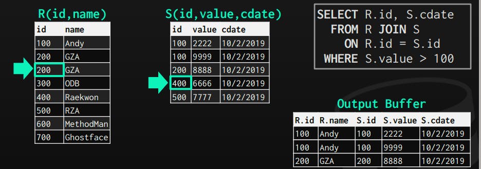
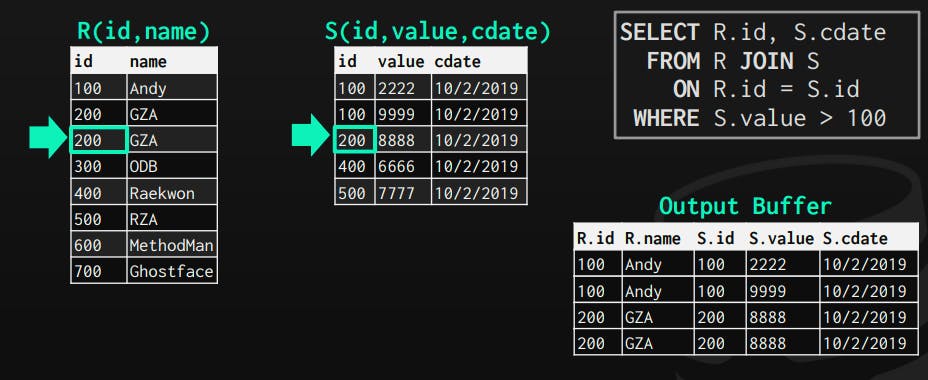
Join Operator Output

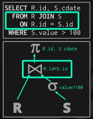
In the given query, the planner noticed that a join is required, thus it inserted a join operator in the query plan. This operator gets its input from both tables R, S. However, its output can vary a lot depending on:

Processing Model
Storage Model
Query itself

1- Data

In this type, the operator outputs the actual data of the record. It does so by copying the whole attributes that it receives (from the previous operator) along with the record that was matched.

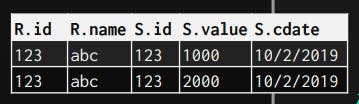
One main advantage of it is that the next operators on the plan, don't need to go back for the pages to get the remaining attributes they may need. This is suitable for row-based databases, as the whole row is stored on the same page continuously. So, the cost of retrieving all attributes is not so huge.

2- RecordIds

In this type, the operator outputs only the RecordIds of the tuples that matched the join, and the next operators on the plan consume them and retrieve only attributes it needs on demand (late-materialization).

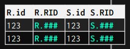
It's ideal for columnar databases because it doesn't fetch pages for attributes that won't be used later in the plan.

Join Operator Algorithms

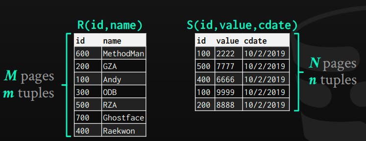
Cost analysis terms used: we will use the R table, which has M pages stored on disk, and m records. S table with N pages on the disk, and n records.

1- Nested Loop Join

* Simple Nested Loop Join

This is the most straightforward algorithm to do joins, just brute-force and output the data.

foreach tuple r in R:
    foreach tuple s in S:
        emit if r and s match

Cost of running R (bigger pages) as an outside table: M + (m*N)

Example dataset where M = 1000, N = 500, m = 100,000, n = 40,000

Cost = 1000 + (100,000 * 500) = 50,001,000 I/Os

Cost of Running S (smaller pages) as an outside table: N + (n*M)

Cost = 500 + (40,000 * 1000) = 40,000,500 I/Os

As we can see, running the smaller table as the outside table makes it run faster (while it's still too slow).

* Block-Nested Loop Join

In this algorithm, we try to reduce page fetches using the same brute force algorithm, but being a little bit smarter about page fetches, maximizing the utilization of each page fetched.

foreach block br in R:
    foreach block bs in S:
        foreach tuple r in br:
            foreach tuple s in bs:
                emit if r and s matches

Cost: M + (M*N) = 1000 + 500*1000 = 501,000 I/Os. It's apparent that there's a huge optimization, the previous one was 50,001,000 I/Os (100x more I/Os)

Again, using the smaller table in terms of pages optimizes this a little bit.

This algorithm becomes better and better if we have a larger buffer, and if we are lucky enough to fit all pages in memory, it will be M+N I/Os.

* Index Nested Loop Join

We can avoid too many sequential scans by an index to find table matches.

foreach tuple r in R:
    foreach tuple s in index(ri = si):
        emit r,s if matches

In this algorithm, we use the outer table which has no index, and the inner which has an index. By doing so, we can search for values using the index instead of doing sequential scans every time we need to find a matching.

Cost: M + (m*C) where C is the cost of searching an index for a specific value, which depends on the implementation of the index.

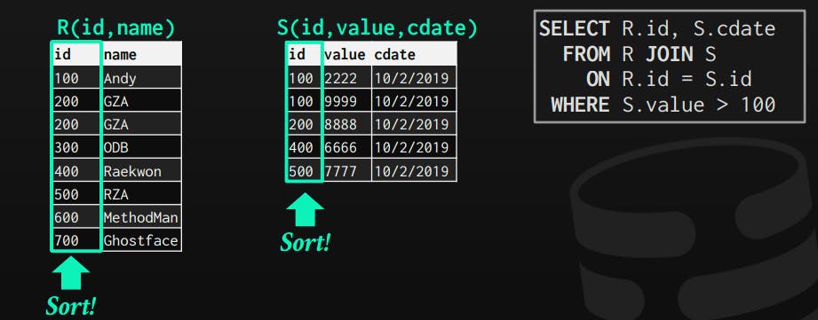
2- Sort-Merge Join

It's basically consisting of two phases:

Phase 1: Sort both tables on the join keys, sorting algorithm can be determined based on whether it fits in memory or not.

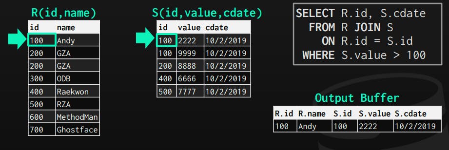
Phase 2: Merge by looping with two cursors, and emit matches only.

sort R, S on join keys
cursorR = firstSortedR, cursorS = firstSortedS
while cursorR and cursorS:
    if cursorR > cursorS:
        increment cursorS
    else if cursorS > cursorR:
        increment cursorR
    else if cursorR matches cursorS:
        emit
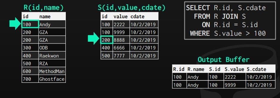
        increment cursorS

Start the matching process

The case when the cursor of s is larger than the cursor of r

Important note: sometimes we might need to backtrack because we might lose some matching if we just skipped to the next without thinking.

In the case when we reach r = 200, we will find a match on s = 200, and by following the algorithm, we will increase s cursor, and it will point to 400.

Now, r cursor will be less than s cursor, so increase it, but eventually, we will find 200 in r cursor again, but at the same time, s cursor is at 400, it might skip and don't return a matching, however, it has a matching that should be included. We can backtrack s cursor to the previous value of 200, to check whether it matches or not.

We need to backtrack

The backtracking here is so simple, only the previously matched value should be backtracked, so it doesn't have a huge impact on the algorithm performance.

Cost: Sort + Merge

Sort(R) = 2M ∙ (1 + ⌈ logB-1 ⌈M / B⌉ ⌉), Sort(S) = 2N ∙ (1 + ⌈ logB-1 ⌈N / B⌉ ⌉)

Merge = M+N

Using sample dataset as previous algorithms, with B buffer pages = 100

Sort(R) = 4000 I/Os, Sort(S) = 2000 I/Os, Merge = 1500 I/Os

Total = 7500 I/Os

It's a lot better than nested loop join!

When it's used?

It's suitable when on or both tables are sorted on the keys (has a tree table), or when the output should be sorted using the matching keys. Also, if there's an existing index on the matching keys, it will remove the cost of sorting as it's already sorted, which makes it much faster.

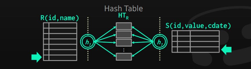
3- Hash Join

Hashing can help us to identify matching, by building a hashtable from one table and using it to find matches.

Phase 1: Build the table, by using the outer table, hash every matching key and store it in the table (if the outer table is smaller, this means less hashtable size)

Phase 2: Probe the table by scanning the inner table, hashing each matching key, and looking at the hashtable to find matches of it.

buld hashtable HTr from R
foreach tuple s in S:
   emit if h(s) in HTr

We can build a bloom filter during the build phase, which indicates when the key is likely not to be in the hash table. In the probe phase, Before each jump on the hash table, we check the bloom filter, if it says it has the key, it's safe to assume it's there, and there's no need to check the hashtable. However, bloom filters produce negative false, which means that it may say that a specific key is not there, but it's in the table. So, we need to look at the hashtable to know precisely.

As a bloom filter is usually small, we can keep it in memory, which reduces I/O.

Cost: 3 (M+N) = 3 * (1000 + 500) = 4500 I/Os. Less than sort-merge.

This cost can be reduced by using static hashing, if DB knows the size of the outer table before starting, which depends on the implementation of the DBMS.

In general, hashing is almost better than sorting when it comes to joining operator, however, it might be worst if data is non-uniform, or we need to sort results before returning. Usually, DBMS use either of them depending on the query.

References

CMU15-445/645 Database Systems lecture notes. Retrieved from: 15445.courses.cs.cmu.edu/fall2019

Note: ChatGPT was used to help me refine and make this post more concise, and readable, and provided some examples. So huge thanks to OpenAI!

Samuel Sorial's Blog